Last Friday and Saturday, the wind here in Punta Arenas was extreme, even for the local standard. It might not have been the perfect time to arrive here via airplane, but on the other hand, the landing was a real experience, something to remember later on. A striking thing about the weather situation was the heavy, stormy wind in connection with bright sunshine. Looking out of the window, you wouldn’t imagine almost being blown off the street when going out for dinner. The wind also wasn’t very cold, so being outside was actually quite enjoyable.

The Centro Meteorologico Maritimo reported a maximum wind speed of 58.2 knots, or 108 km/h. On social media, people shared the experiences they had with the unusually strong wind: Windows were broken and power outages were reported in parts of the city. Someone uploaded a video from an airplane landing on Saturday, in which one can see a little bit of the swaying of the plane, followed by a rather rough landing.

Lots of flights were canceled on Saturday and consequently, there was a big chaos at the airport. This complicated retrieving my suitcase, which was lost the day before when I flew to Punta Arenas. Luckily, the baggage (which contained some important cables and switches needed for the site) was there on Saturday.

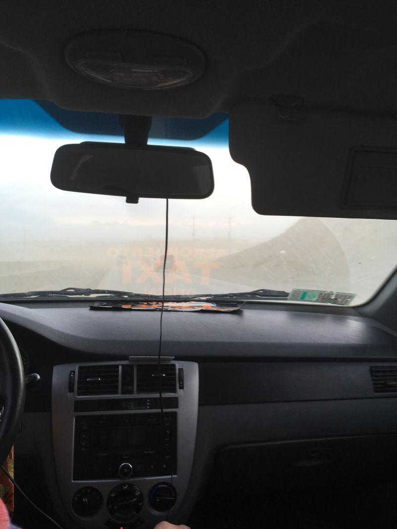
The wind raised quite a lot of dust, which complicated car traffic in addition to the heavy wind gusts. So on top of having to steer against the wind, the view was also obstructed by a thick dust plume from time to time. A truck besides the road was actually overturned. Riding the taxi on the way from/ to the airport was quite exciting:

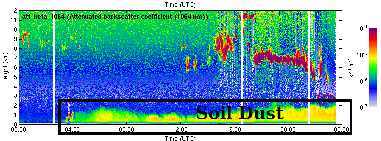
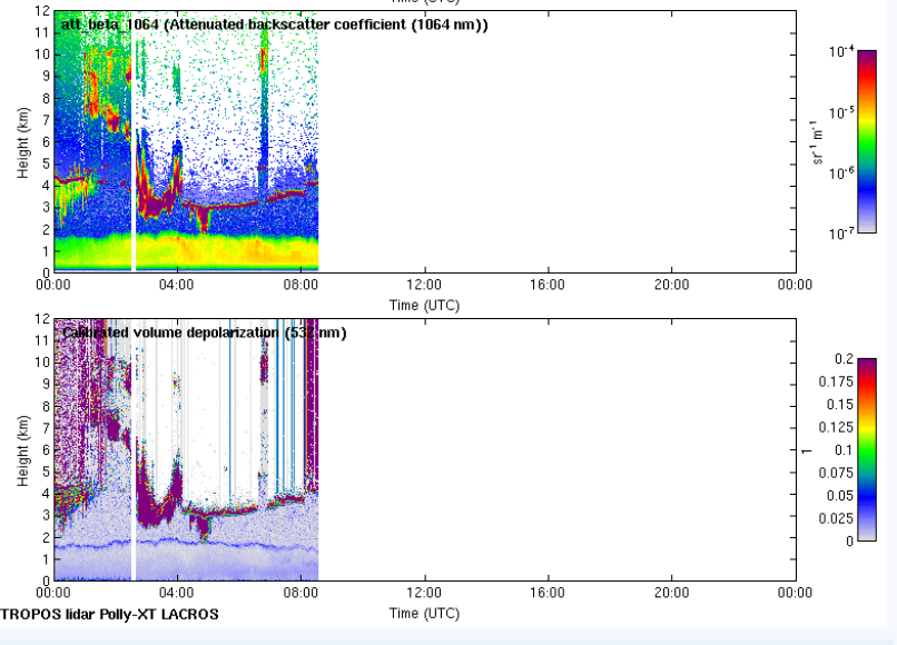
We can also see this dust in our lidar data. The dust stays in the lower atmosphere, below 2 km altitude, as can be seen in the POLLY backscatter (1064 nm).

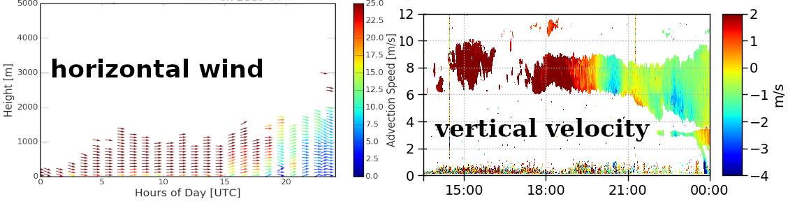
When checking our remote sensing data, we noticed that we cracked some of the standard color scales in our quicklook plots: The Shaun wind lidar quick look plots show only dark red arrows during the first half of February 16, starting in the second height bin. Below, surface friction slows down the wind at least a little bit so that it’s “only” around 20 m/s, or 70 km/h. Shaun measures the horizontal and vertical wind. In the graph below, the left panel shows the horizotal wind. Vertical wind was exceptionally high as well, which can be seen in the radar data: The Doppler velocity, which can be translated to the combined vertical wind + fall velocity of cloud particles, is shown in the left panel below. Also here, the color scale is not wide enough to accommodate the vertical wind speeds of sometimes almost 4 m/s:

Both graphs show the time on the horizontal axis and the height in the vertical coordinate. The color scale depicts the wind speed. Red means very high wind velocities.

[TV]

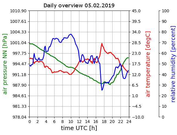
During the first days of this week, we had quite special meteorological conditions at Punta Arenas. Persistent wind from the north brought unusually warm air to the Magallanes region. Together with the absence of clouds and hence strong heating by the sun, surface temperatures climbed to extraordinarily high values. On Monday (4 Feb), the maximum temperature at Punta Arenas airport reached almost 25°C and on Tuesday the maximum was 28°C. Long-term temperature records were set for several other stations throughout the region, as for example Porvenir and Puerto Natales with both above 30°C (https://twitter.com/meteochile_dmc/status/1092808761167831040). On Tuesday evening, the heat period came to a sudden end, when a cold front arrived. This is nicely visible in the surface observation (at the UMAG roof platform, shown below) as temperature drops by 15°C (red curve) and pressure increases (green curve) after 17:30 UTC (14:30 local). A nice feature is also the jump in temperature and drop in relative humidity (blue curve) directly before the front, which is probably caused by Föhn effects as the wind increased and backed toward westerly directions.

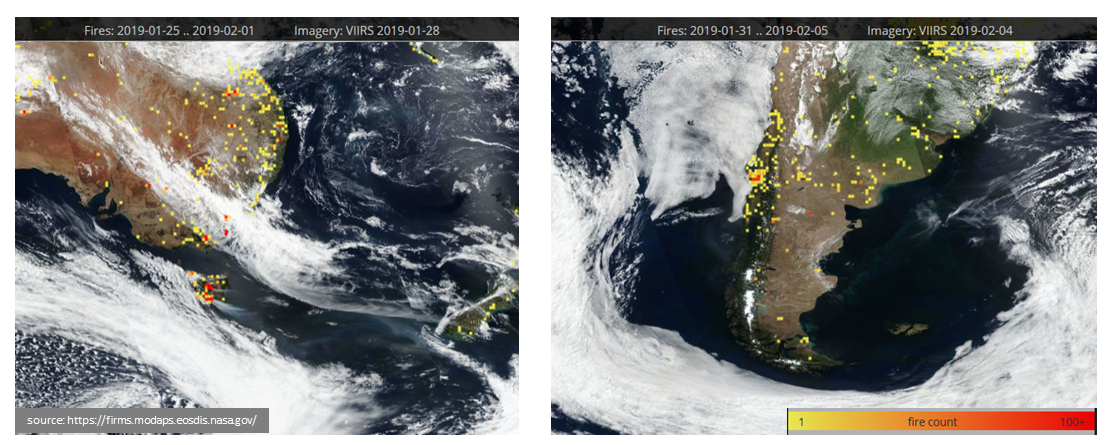
But the airmass from the north did not only bring high temperatures, but aerosol as well. Our lidar PollyXT (see also prior blog posts here and here) detected several lofted layers between 1 and 5km height on Monday and Tuesday. Several plumes are visible in the backscatter signal. One with rather weak backscatter and low depolarization ratio on Tuesday and another one with higher backscatter and some features with higher depolarization ratio.

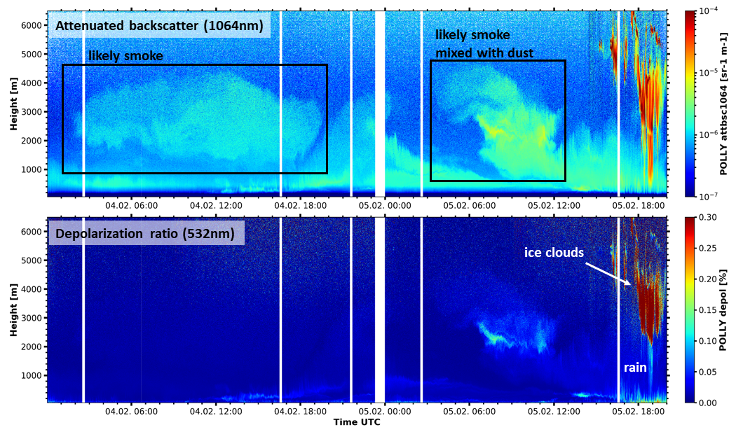
The aerosol optical depth, a measure for total aerosol load in the atmosphere, reached values up to 0.1 (at a wavelength of 500nm). The spectral dependence between 440 and 870nm (called Ångström exponent) was around 1.5, indicating predominantly small particles with a diameter well below 1μm. Based on their optical parameters these particles are most likely smoke caused by wildfires, on Tuesday maybe mixed with some soil dust.

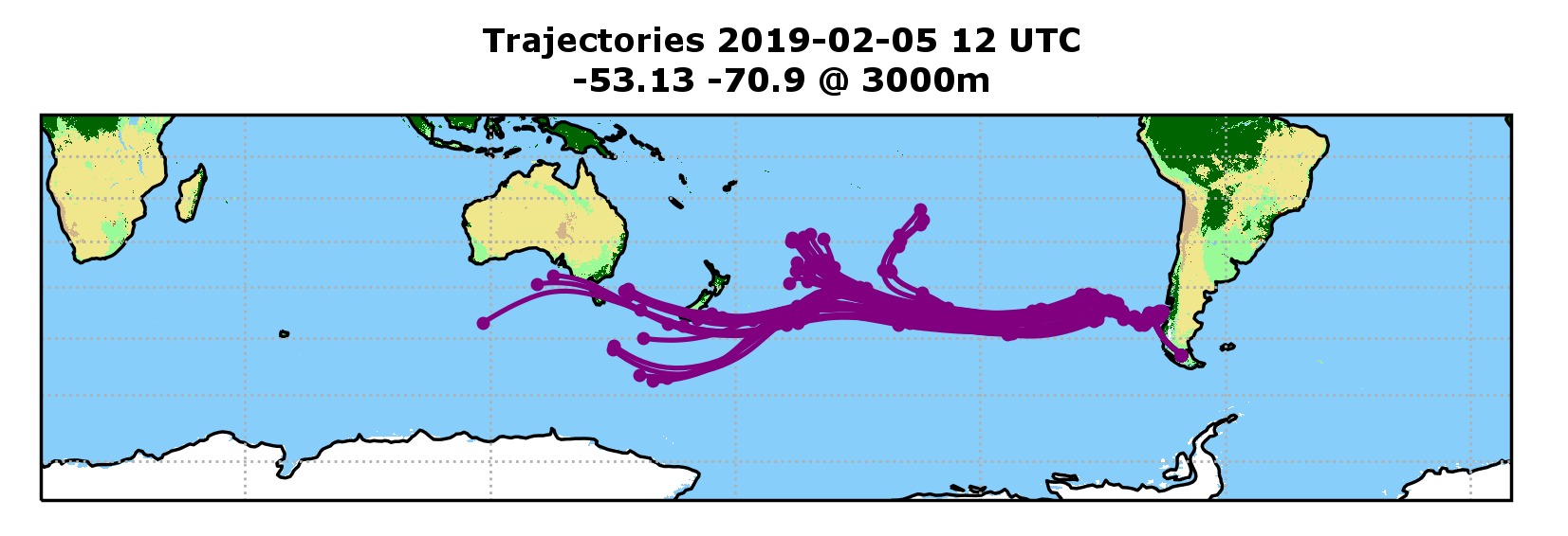
We were not yet able to pin-down the source of this aerosol plume unambiguously. Two source regions are possible: either the forest fires in the Region of Araucanía in Chile or the fires on Tasmania, Australia. Simulations with the HySPLIT (https://www.ready.noaa.gov/HYSPLIT.php) trajectory model (a model that traces the pathway of air parcels), show that the airmass, which was at Punta Arenas in 3km height on Tuesday 12 UTC (9 local) crossed both region during the prior 10 days. We are thus looking forward to have to solve yet another research puzzle.

[mr]

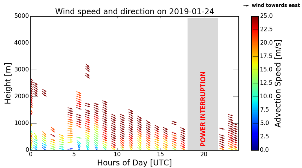
On Thursday evening, LACROS was struck by a power failure that affected the whole university. After almost 3 hours electricity was available again and we were able to put most instruments operational again right after the incidence. The cloud radar MIRA required some more attention by the on-site personal and the remote support from Leipzig. On Friday, we could narrow down the problems to an ethernet connector. Let us hope that the backup connection will work until we can fix the problem. 

The cause for this interruption were very strong winds during the whole day. A low-pressure system over Drake street triggered west-north-westerly flow at Punta Arenas. Supported by the terrain, this situation seems to favor strong surface winds at the city. Below you can see the observations of our scanning Doppler lidar, which (among other things) can measure profiles of horizontal wind velocity and direction. As the signal requires the presence of particles, that scatter the light back to the instrument. Hence, continuous information is usually constrained to the boundary layer – the layer of the atmosphere, which is directly coupled to the ground and contains comparably high amounts of aerosols.  Shown is a time-height series of the full day. Above 700 m the strong winds persisted the whole day, but affected ground only at around 10 UTC (7 local) and after 17 UTC (14 local).

The strongest gusts at the ground reached 107km/h in the city and 117km/h at the harbor. The local newspaper also reported on this issue: https://laprensaaustral.cl/titular1/temporal-de-viento-dejo-multiples-estragos-en-punta-arenas/

[mr]

Happy new year everybody. I'd like to point your attention to the Polly-XT measurements of clouds and aerosol taken in the morning of 10 January 2019.

Below you see a nice quicklook created from PollyXT data. Besides cloud layers at all heights above 2 km, a pronounced planetary boundary layer (PBL) is visible at heights below 2 km. This is nicely shown in the upper panel in the Figure below that shows the attenuated backscatter coefficient observed at 1064 nm. A look at the lower panel, showing the 532-nm volume depolarization ratio, indicates the presence of a depolarizing layer at the top of the PBL. This is according to recent studies of TROPOS dried sea salt aerosol, containing crystallized salt particles. Their non-sphericity causes a certain degree of depolarization to the backscattered light.

It is also worth looking at the observed cloud layers: between 0500 and 0800 UTC the cloud layer at 3-4 km height does not produce any ice particles, even though temperatures at cloud top (detected by the cloud radar, not seen by the lidar) where below -8 to -10 °C.

[PS]

After finishing the setup, we are now at normal campaign mode and all the instruments are observing 24/7 (see the previous blog post for details about locations of the quicklooks). Now it’s the time to have a look in the data collected so far. Let’s start with the PollyXT lidar.

PollyXT emits short pulses of light at a repetition frequency of 20 Hz. The light of each pulse hits particles in the atmosphere, for example air molecules, aerosol particles or clouds and is eventually scattered back to the lidar. The returned light is collected by a receiver (that counts single photons). By the time of travel between pulse emission and reception of the returned photons, the height of the scattering particles can be determined. As a result, a vertical profile of the number of photons scatted back from each height level is obtained. One profile is assembled from a series of 600 laser pulses, which corresponds to a temporal resolution of 30 s. The collected profiles are here visualized as a time-height cross section of the atmosphere above the instrument.

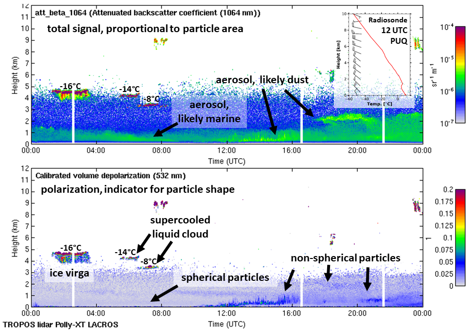
The example above shows a time-height cross section one of our first observations over Punta Arenas for the full day of the 28 November 2018. In the upper panel the total signal for a certain channel is shown, which is roughly proportional to the size of the particles. A lot signal was detected in the boundary layer up to 1.5 km height. As this layer is directly coupled to the surface, there is usually a high aerosol load. Later that day, the boundary height increases up to 2.8 km height and some more distinct layers were present. Between 1 and 8 UTC a couple of layered clouds was detected between 3 and 5 km. In addition to the total signal, the polarization state of the returned signal is analyzed. This quantity is called depolarization ratio, as it compares, the polarization direction of the emitted pulse with one of the received signal. This depolarization ratio helps to characterize the shape of the observed particles. The particles in the boundary layer until 11 UTC show almost no depolarization. Hence, they are spherical, which is typical for marine aerosol. Later, higher depolarization ratios indicate the presence of non-spherical particles in the boundary layer, which is a hint for soil dust.

We can also obtain more information about the clouds using the depolarization ratio. To understand this, we need some basic insights into cloud microphysics: In the atmosphere, liquid water can exist down to -38°C, because thermodynamics cause a high energy barrier when going from liquid to solid phase. If you try to freeze water in your fridge, the walls of the box help to lower this energy and freezing may occur at ‘high’ temperatures. In the atmosphere, the same job might be done by aerosol particles, which are then called ice-nucleating particles. Their efficiency depends strongly on temperature – the colder the more aerosol particles can act as ice nucleating particles. In our case here, the highest and therefore coldest cloud produces ice, nicely visible as an ice virga falling out of the liquid layer. The other two clouds are a little bit lower and warmer and do not form ice. In the case shown, we added temperature information for each cloud, taken from a radiosonde launch performed at Punta Arenas airport at 12 UTC. As can be seen, the highest cloud layer, with a temperature of -16°C  formed ice. The two lower cloud layers contained only supercooled liquid water droplets.

One major target of DACAPO PESO is to investigate the above described phenomena of ice formation in liquid clouds in the pristine environment of the southern mid-latitudes compared to the more aerosol laden northern hemisphere.

 [mr]

Three weeks passed since the first instruments where switched on around 26 November. Even though the actual hardware implementation did not take much more than 3 days, all members of the DACAPO-PESO team are working hard on getting the processing chain for the data up and running.

It was decided to implement a two-stage data processing. First processing is done on a server on-site in Punta Arenas. One 120-TB machine collects all data from the individual instruments of LACROS and frequent quicklooks are created. During night time, when network traffic at UMAG is low, most data is being transferred to the central remote sensing server of TROPOS in Leipzig. Only the raw spectra of 35-GHz radar is excluded from this data transfer.

Everybody is invited to have a look at the quicklooks of the DACAPO-PESO observations. Below is a list of links to most of the measurement quicklooks.

• Observations of the Raman Polarization lidar Polly-XT: http://polly.tropos.de/
• Cloudnet-processed data of LACROS: http://lacros.rsd.tropos.de/cloudnet/cloudnet.php
• Quicklooks of the indivdual instruments: http://lacros.rsd.tropos.de/cloudnet/punta-arenas_ql.php