After finishing the setup, we are now at normal campaign mode and all the instruments are observing 24/7 (see the previous blog post for details about locations of the quicklooks). Now it’s the time to have a look in the data collected so far. Let’s start with the PollyXT lidar.

PollyXT emits short pulses of light at a repetition frequency of 20 Hz. The light of each pulse hits particles in the atmosphere, for example air molecules, aerosol particles or clouds and is eventually scattered back to the lidar. The returned light is collected by a receiver (that counts single photons). By the time of travel between pulse emission and reception of the returned photons, the height of the scattering particles can be determined. As a result, a vertical profile of the number of photons scatted back from each height level is obtained. One profile is assembled from a series of 600 laser pulses, which corresponds to a temporal resolution of 30 s. The collected profiles are here visualized as a time-height cross section of the atmosphere above the instrument.

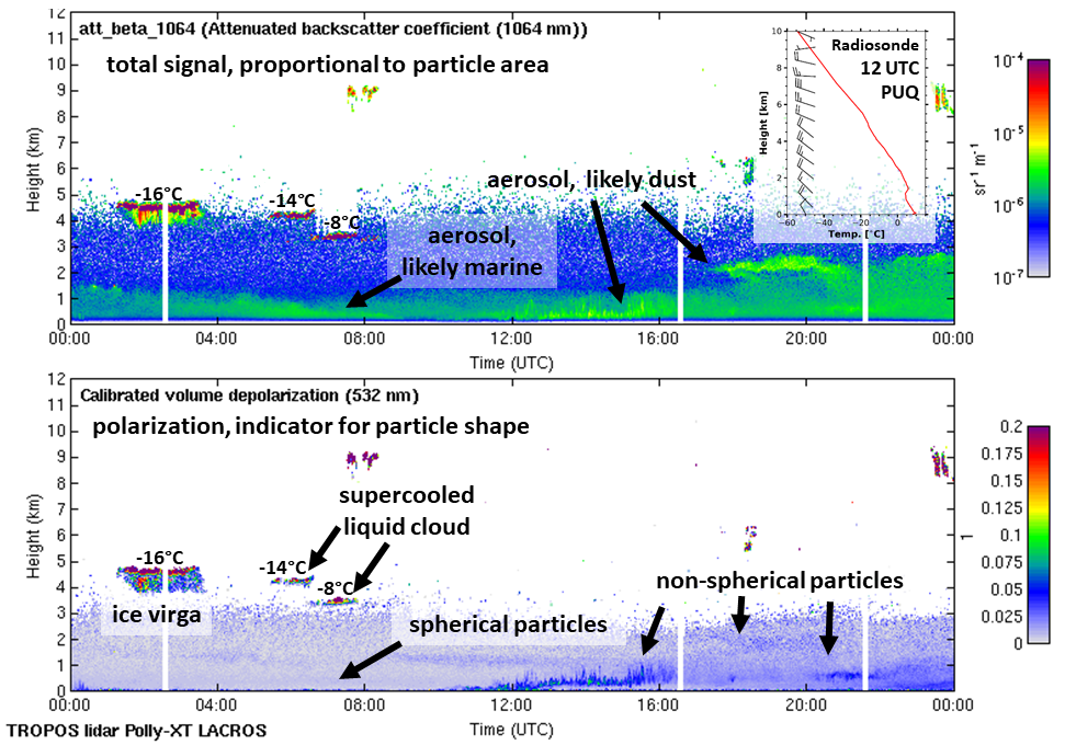
The example above shows a time-height cross section one of our first observations over Punta Arenas for the full day of the 28 November 2018. In the upper panel the total signal for a certain channel is shown, which is roughly proportional to the size of the particles. A lot signal was detected in the boundary layer up to 1.5 km height. As this layer is directly coupled to the surface, there is usually a high aerosol load. Later that day, the boundary height increases up to 2.8 km height and some more distinct layers were present. Between 1 and 8 UTC a couple of layered clouds was detected between 3 and 5 km. In addition to the total signal, the polarization state of the returned signal is analyzed. This quantity is called depolarization ratio, as it compares, the polarization direction of the emitted pulse with one of the received signal. This depolarization ratio helps to characterize the shape of the observed particles. The particles in the boundary layer until 11 UTC show almost no depolarization. Hence, they are spherical, which is typical for marine aerosol. Later, higher depolarization ratios indicate the presence of non-spherical particles in the boundary layer, which is a hint for soil dust.

We can also obtain more information about the clouds using the depolarization ratio. To understand this, we need some basic insights into cloud microphysics: In the atmosphere, liquid water can exist down to -38°C, because thermodynamics cause a high energy barrier when going from liquid to solid phase. If you try to freeze water in your fridge, the walls of the box help to lower this energy and freezing may occur at ‘high’ temperatures. In the atmosphere, the same job might be done by aerosol particles, which are then called ice-nucleating particles. Their efficiency depends strongly on temperature – the colder the more aerosol particles can act as ice nucleating particles. In our case here, the highest and therefore coldest cloud produces ice, nicely visible as an ice virga falling out of the liquid layer. The other two clouds are a little bit lower and warmer and do not form ice. In the case shown, we added temperature information for each cloud, taken from a radiosonde launch performed at Punta Arenas airport at 12 UTC. As can be seen, the highest cloud layer, with a temperature of -16°C  formed ice. The two lower cloud layers contained only supercooled liquid water droplets.

One major target of DACAPO PESO is to investigate the above described phenomena of ice formation in liquid clouds in the pristine environment of the southern mid-latitudes compared to the more aerosol laden northern hemisphere.

 [mr]